Create a PivotTable to analyze worksheet data

Mastering PivotTables in Excel: A Comprehensive Guide

Welcome to the ultimate guide to PivotTables in Excel! Whether you’re using Windows or macOS, this tutorial will empower you with the skills to effortlessly create, customize, and manage PivotTables, turning your raw data into meaningful insights.

Objectives:

1. Windows Wonder: Learn the step-by-step process of crafting a PivotTable in Excel for Windows. From selecting data to defining the data source, this section ensures you harness the power of PivotTables efficiently.
2. macOS Mastery: Mac users, fear not! This part of the tutorial is dedicated to guiding you through the process of creating PivotTables on your macOS device. From data selection to customization, we’ve got you covered.
3. Diverse Sources: Dive deeper into PivotTable versatility. Explore alternative sources beyond traditional tables or ranges. Whether it’s external data, Data Model integration, or Power BI, discover how to broaden your PivotTable horizons.
4. Constructing Your PivotTable: Once you’ve selected your data, it’s time to build your PivotTable. This section provides insights into adding and organizing fields effortlessly, ensuring your PivotTable aligns with your analytical goals.
5. Updating Your PivotTables: Keep your analyses up-to-date with ease. Learn the art of refreshing PivotTables, whether you have a single table or multiple PivotTables in your workbook.
6. Managing PivotTable Values: Dive into advanced options for manipulating how your PivotTable values are presented. From summarizing values to showcasing data as percentages, these tips will enhance your data representation.
7. Deleting a PivotTable: Ready to bid farewell to a PivotTable? Learn the straightforward steps to remove it without disrupting your overall Excel setup.
8. Effective Data Formatting: Before delving into PivotTables, ensure your data is formatted for success. This quick guide provides tips on achieving tabular excellence, maintaining header harmony, and utilizing powerful data handling with Power Query.

By the end of this tutorial, you’ll not only be a PivotTable pro but also equipped with data formatting best practices. Let’s embark on this journey to unlock the true potential of Excel. Ready to elevate your data game? Let’s dive in!

Windows

Crafting a PivotTable in Excel for Windows: A Quick Guide

Ready to harness the power of PivotTables in Excel for Windows? Follow these simple steps to effortlessly create a PivotTable from your data.

• Select Your Data: Begin by choosing the cells containing the data you want to pivot. Ensure that your data is structured with columns and a single header row. Refer to the Data format tips and tricks section for additional insights.

• Access PivotTable Options: Navigate to the Insert tab and click on PivotTable.This action initiates the creation of a PivotTable based on your selected data.

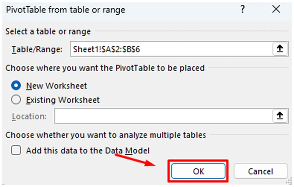
• Define the Data Source: A window will appear where you can choose the location of the PivotTable report. Opt for New Worksheet to place the PivotTable in a new worksheet, or choose Existing Worksheet to specify the location on an existing sheet.Note:
  • If you select Add this data to the Data Model, the table or range used for the PivotTable will be integrated into the workbook’s Data Model. This option offers additional functionality; explore more about it.

• Finalize and Confirm: After making your selections, click OK to create the PivotTable.

Exploring Different Sources for PivotTables in Excel

In Excel, creating PivotTables is a versatile process that extends beyond traditional tables or ranges. Let’s delve into alternative sources you can utilize for your PivotTables.

• Diverse Sources: Click the down arrow on the button to uncover a range of potential sources for your PivotTable. Beyond the standard use of an existing table or range, Excel offers three additional sources to enrich your PivotTable experience.
  • Note: Depending on your organization’s IT settings, you may spot your organization’s name in the list, such as “From Power BI (Microsoft).”

• External Data Source: Opt for this option to bring in data from an external source, broadening your possibilities beyond internal datasets.

• Data Model Integration: If your workbook incorporates a Data Model, choose this option. It’s ideal for creating PivotTables from multiple tables, introducing custom measures, or handling extensive datasets.

• Power BI Integration: Select this option if your organization utilizes Power BI. It allows you to explore and connect to approved cloud datasets accessible to you.

Constructing Your PivotTable in Excel

Creating a PivotTable in Excel is a breeze. Follow these steps to add and organize fields effortlessly.

• Add a Field: In the PivotTables Fields pane, tick the checkbox next to the field name that you want to add to your PivotTable.Note: Selected fields automatically go to their default areas—non-numeric fields land in Rows, date, and time hierarchies find their place in Columns, and numeric fields snugly fit into Values.

• Adjust Field Placement: To relocate a field from one area to another, simply drag the field to your desired target area.

Updating Your PivotTables in Excel

Keeping your PivotTables up-to-date is crucial, especially when new data is added to your data source. Here’s how you can effortlessly refresh your PivotTables in Excel.

• Refresh a Single PivotTable: Right-click anywhere within the PivotTable range that needs updating. Choose “Refresh” from the menu.
• Refresh Multiple PivotTables: If you have several PivotTables, start by selecting any cell in any PivotTable. Navigate to the ribbon and go to PivotTable Analyze. Click the arrow under the Refresh button and choose “Refresh All.”

Managing PivotTable Values in Excel

Effortlessly manipulate how your PivotTable values are presented with these practical tips.

• Summarize Values By: By default, values in the PivotTable’s Values area appear as a SUM. If Excel interprets your data as text, it displays as a COUNT. Ensure data types match for accurate results. Adjust the default calculation by selecting the arrow next to the field name and choosing “Value Field Settings.”

Modify the calculation in the “Summarize Values By” section. Excel may automatically add it in the Custom Name section, like “Sum of FieldName,” but customization is possible. Utilize Number Format to adjust the entire field’s format. Tip: Avoid renaming PivotTable fields until setup is complete. Use Find & Replace (Ctrl+H) to replace “Sum of” with a blank field.

• Show Values As: Instead of summarizing data through calculation, showcase it as a percentage of a field. For instance, display household expenses as a % of Grand Total instead of their sum. Open the Value Field Setting dialog box and navigate to the “Show Values As” tab to make selections. Display a Value as Both a Calculation and Percentage: Drag the item into the Values section twice. Adjust the “Summarize Values By” and “Show Values As” options for each.

Web

Creating a PivotTable in Excel: A Quick Guide

Effortlessly organize and analyze your data with a PivotTable in Excel. Follow these steps:

• Select Your Data: Highlight the table or data range in your sheet.

• Open Insert PivotTable: Go to Insert > PivotTable to open the Insert PivotTable pane.

• Choose Creation Method: Decide whether to manually create your PivotTable or use a recommended one. Here’s how:
  • For Your Own PivotTable: On the “Create your own PivotTable” card, choose either “New sheet” or “Existing sheet” as the destination for your PivotTable.For a Recommended PivotTable: On a recommended PivotTable, also select either “New sheet” or “Existing sheet” for the PivotTable destination.

Note: Recommended PivotTables are exclusively available to Microsoft 365 subscribers.

Exploring Different Sources for PivotTables in Excel

In Excel, creating PivotTables is a versatile process that extends beyond traditional tables or ranges. Let’s delve into alternative sources you can utilize for your PivotTables.

• Diverse Sources: Click the down arrow on the button to uncover a range of potential sources for your PivotTable. Beyond the standard use of an existing table or range, Excel offers three additional sources to enrich your PivotTable experience.
  • Note: Depending on your organization’s IT settings, you may spot your organization’s name in the list, such as “From Power BI (Microsoft).”

• External Data Source: Opt for this option to bring in data from an external source, broadening your possibilities beyond internal datasets.

• Data Model Integration: If your workbook incorporates a Data Model, choose this option. It’s ideal for creating PivotTables from multiple tables, introducing custom measures, or handling extensive datasets.

• Power BI Integration: Select this option if your organization utilizes Power BI. It allows you to explore and connect to approved cloud datasets accessible to you.

Effortless PivotTable Customization in Excel

Streamline your data presentation with these simple steps using the PivotTable Fields pane:

• Access the PivotTable Fields Pane: Head to the PivotTable Fields pane and check the box next to each field you wish to incorporate into your PivotTable.
• Default Placement: Automatically, non-numeric fields seamlessly integrate into the Rows area, while date and time fields effortlessly find their spot in the Columns area. Numeric fields naturally slot into the Values area.
• Manual Arrangement: Take control of your data arrangement by manually dragging and dropping any available item into your preferred PivotTable field. If there’s an item you wish to remove, a simple drag out from the list or unchecking it does the trick.

Optimizing PivotTable Values in Excel

Refine your data representation effortlessly with these steps:

Summarizing Values By:

By default, Values in the PivotTable are presented as a SUM, unless Excel identifies the data as text, in which case it appears as a COUNT. It’s crucial to maintain consistency in data types for accurate results.

To change the default calculation, right-click any value in the row and choose the “Summarize Values By” option.

Show Values As:

Explore alternative presentations by displaying values as a percentage of a specific field. For instance, transform household expenses into a percentage of the Grand Total rather than a simple sum.

1. Right-click any value in the column you want to modify.
2. Select “Show Values As” from the menu, revealing a list of available options.
3. Make your selection from the list.

For a percentage of the Parent Total, hover over the desired item in the list and choose the parent field as the basis for the calculation. Excel provides flexibility in data interpretation, ensuring your insights are tailored to your needs.

Refreshing PivotTables:

When you introduce new data to your PivotTable data source, it’s essential to refresh any corresponding PivotTables. Follow these easy steps:

1. Right-click anywhere within the PivotTable range.
2. Select “Refresh” from the menu.

This ensures that your PivotTables dynamically incorporate any changes in the underlying data source, maintaining accuracy and relevancy in your analyses.

Deleting a PivotTable in Excel

If you’ve decided to part ways with a PivotTable, here’s a straightforward guide on how to bid it farewell:

Option 1: Delete PivotTable Range

1. Select the entire range of your PivotTable.
2. Press the “Delete” key.

This action won’t impact other data, PivotTables, or charts in the vicinity.

Option 2: Delete the Sheet (if applicable)

If your PivotTable resides on a standalone sheet with no essential data:

1. Right-click on the sheet containing the PivotTable.
2. Choose “Delete.”

By opting for either method, you can swiftly remove the PivotTable without disrupting your overall Excel setup.

Mac

Preparing for PivotTables: Quick Guide

Before diving into PivotTables, make sure your data is set up for seamless analysis. Here’s a brief checklist:

• Organized Tabular Format:

• Ensure your data is structured in a tabular format.
• No blank rows or columns should disrupt the flow.

2. Excel Tables Advantage:

• Consider using Excel tables for your data.
• Tables automatically incorporate new rows and columns upon data refresh.

3. Uniform Data Types:

• Maintain consistency in data types within columns.
• Avoid mixing dates and text within the same column.

4. Snapshot with PivotTables:

• PivotTables operate on a data snapshot known as the cache.
• Rest assured, your actual data remains unchanged.

Creating a PivotTable Made Easy: Recommended Approach

For those new to PivotTables or seeking a hassle-free start, the Recommended PivotTable feature is your go-to. Excel takes the reins, intelligently organizing your data into a PivotTable layout that makes sense. It serves as a launching pad for further customization. Once the Recommended PivotTable is generated, feel free to experiment with different field arrangements to achieve your desired outcome. If you’re looking for an interactive guide, check out our “Make your first PivotTable” tutorial.

Step-by-Step Guide:

• Click on any cell within your source data or table range.

• Navigate to Insert > Recommended PivotTable.

• Let Excel work its magic, presenting you with various options based on your data, as illustrated in this example using household expense data.
• Choose the PivotTable layout that suits your preference and click OK. Excel promptly creates a PivotTable on a new sheet, unveiling the PivotTable Fields list for further adjustments.

Creating a PivotTable: Step-by-Step Manual Method

When it comes to hands-on PivotTable creation, you’re in control. Follow these straightforward steps:

• Click on any cell within your source data or table range.

• Navigate to Insert > PivotTable. (This option is found in the Data tab, under the Analysis group.)

• Excel presents the Create PivotTable dialog box, with your range or table name already highlighted. For our example, we’re using a table named “tbl_HouseholdExpenses.”
• In the “Choose where you want the PivotTable report to be placed” section, decide whether you want it on a New Worksheet or an Existing Worksheet. If you choose the latter, specify the cell for the PivotTable.

• Click OK, and voila! Excel generates a blank PivotTable, ready for your input, and showcases the PivotTable Fields list.

Now, you’re set to tailor your PivotTable to meet your specific needs. Dive into the PivotTable Fields list and start shaping your data.

Navigating the PivotTable Fields List

Mastering the PivotTable Fields list is your key to unlocking the potential of your data. Here’s how to effortlessly work with it:

PivotTable Fields List

At the top, in the Field Name section, simply check the box next to the field you wish to incorporate into your PivotTable. By default, non-numeric fields find their place in the Rows area, date and time fields snug into the Columns area, and numeric fields settle in the Values area.

Feel the power of control as you manually drag-and-drop any available item into the desired section of your PivotTable. If you find an item surplus to requirements, a quick drag out of the Fields list or a simple uncheck will do the trick. The flexibility to rearrange Field items is one of the user-friendly features that makes transforming your PivotTable’s appearance a breeze.

Embrace the ease of crafting your PivotTable as you navigate through the Fields list – your gateway to data customization.

Enhancing Your PivotTable: Unveiling Advanced Options

Unveil the potential of your PivotTable with these advanced options:

Summarize By

By default, the Values area in PivotTable displays the sum of data. Be cautious with data types – text data may appear as a count. To modify, click the arrow next to the field name, then choose Field Settings.

In the “Summarize by” section, adjust the calculation method. Note that Excel adds it in the Custom Name section, e.g., “Sum of FieldName,” but you can edit it. If you opt for Number…, you can modify the number format for the entire field.

Pro Tip: Hold off renaming your PivotTable fields until the setup is complete. Use Replace (Edit menu) > Find “Sum of” > Replace with blank for a quick, comprehensive update.

Show Data As

Rather than relying on calculations, showcase data as a percentage of a field. For instance, transform household expenses to a % of Grand Total instead of a simple sum.

Once in the Field Settings dialog box, head to the Show Data As tab to make your selections.

Display both calculation and percentage.

Duplicate the item in the Values section, right-click the value, choose Field Settings, and then set Summarize By and Show Data As options for each. Unlock the full potential of your PivotTable with these advanced features.

Refreshing Your PivotTable: Keep Your Data Current

Ensuring your PivotTable reflects the latest data is crucial. Here’s how you can refresh it effortlessly:

If you’ve added new data to your PivotTable source, follow these steps:

• Single PivotTable Refresh:
  • Right-click anywhere within the PivotTable range.
  • Choose “Refresh.”

• Multiple PivotTable Refresh:
  • Click any cell in any PivotTable.
  • Navigate to PivotTable Analyze on the ribbon.
  • Select the arrow under the Refresh button.
  • Click “Refresh All.”

Stay up-to-date with your data by making these simple yet effective refresh maneuvers. Keep your PivotTable current and accurate with just a few clicks.

Removing a PivotTable: Streamlining Your Data

Sometimes, you might want to declutter your workspace by removing a PivotTable. Here’s how you can do it seamlessly:

If you’ve created a PivotTable and wish to bid it farewell:

• Entire PivotTable Deletion:
  • Highlight the complete PivotTable range.
  • Press the “Delete” key.

• Sheet Deletion (if PivotTable is on a separate sheet):
  • If the PivotTable resides on a sheet with no crucial data:
    • Right-click on the sheet tab.
    • Choose “Delete.”

By following these steps, you can swiftly eliminate a PivotTable, clearing up your workspace without impacting other data or visual elements. Keep your data presentation precise and clutter-free.

Effective Data Formatting: A Quick Guide

Achieving optimal results in Excel begins with smart data formatting. Here are some tips and tricks:

• Tabular Excellence:
  • Ensure your data is in a clean, tabular format.
  • Organize information in columns rather than rows for a structured layout.
• Header Harmony:
  • All columns should boast clear headers.Use a single row with unique, non-blank labels for each column.Steer clear of double rows of headers or merged cells for simplicity.

• Tabular Transformation (Optional):
  • Consider formatting your data as an Excel table for enhanced organization.
  • Navigate to your data, then select “Insert > Table” from the ribbon.

• Powerful Data Handling with Power Query:
  • For intricate or nested data, leverage Power Query.
  • Transform data structures, such as unpivoting, to streamline it into columns with a single header row.

Adopting these practices ensures your data is not just organized but optimized for efficient processing in Excel.