Create a Drop-Down List in Excel

Empower Your Excel Skills: Creating Drop-Down Lists Made Easy

Greetings! Today, let’s unravel the magic of making your Excel sheets more interactive and efficient by incorporating drop-down lists. This nifty technique is a game-changer for data entry, ensuring precision and consistency – a true blessing for anyone dealing with substantial data.

Objectives:

• Also read How to Get Up to RM360 Cashback with Shopee, Grab, and BigPay

1. Windows Wonder: Learn how to prepare your drop-down list, sort your data, and seamlessly implement the list on Windows. Discover the benefits of using an Excel table for enhanced efficiency.
2. macOS Mastery: Speed up your data entry process on macOS by creating and utilizing drop-down lists. This guide will walk you through the steps to restrict data entry effectively.
3. Input Enhancements: Understand additional configurations such as input messages and error alerts for an enriched data entry experience.
4. Quick Reference Guide: A concise summary for both Windows and macOS users, ensuring you have a handy reference for creating drop-down lists whenever you need it.
5. Bonus Tips: Uncover bonus tips, including customizing error messages, to tackle invalid data inputs like a pro.

Let’s dive into the tutorial and master the art of creating drop-down lists in Excel. Whether you’re a seasoned pro or a beginner, these steps are tailored to simplify your data entry processes. Stay tuned for more tech tips and tricks, specifically crafted for our Malaysian audience, here at GajetHQ. See you on the tech side!

Windows

• Prepare Your List: In a new worksheet, type the entries you want in your drop-down list. It’s even better if you organize your list in an Excel table. Quickly convert your list to a table by selecting any cell in the range and pressing Ctrl+T.Why use a table? When your data is in a table, any changes to the list, whether additions or removals, will automatically update associated drop-downs. No extra effort required.

• Sort Your Data: This is an opportune moment to sort your data in the range or table you’re using for your drop-down list.
• Select the Cell: Choose the cell in the worksheet where you want the drop-down list.
• Access Data Validation: Go to the Data tab on the Ribbon, and then select Data Validation.Note: If Data Validation isn’t selectable, your worksheet might be protected or shared. Unlock specific areas of a protected workbook or stop sharing the worksheet before trying again.

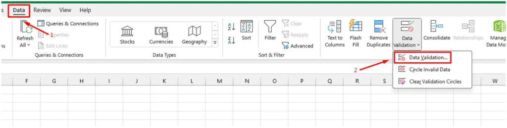
• Configure Data Validation: On the Settings tab, in the Allow box, choose List. In the Source box, select your list range (e.g., A2:A9 on a sheet named Cities, excluding the header row).
• If leaving the cell empty is acceptable, check the Ignore blank box.

• Check the In-cell dropdown box.

• Set Input Message (Optional): Switch to the Input Message tab. If you want a message to appear when the cell is selected, check the Show input message when the cell is selected box. Type a title and message (up to 225 characters). If no message is needed, clear the checkbox.

• Configure Error Alert (Optional): Move to the Error Alert tab. If you want a message to pop up when someone enters something not in the list, check the Show error alert after invalid data is entered box. Choose a style from the box and type a title and message. If no message is required, clear the checkbox.Not sure about the Style box?

• To allow entering data not in the drop-down list, choose Information or Warning.To restrict entering data not in the list, select Stop.

Note: Without a title or text, the default title is “Microsoft Excel,” and the message is: “The value you entered is not valid. A user has restricted values that can be entered into this cell.”

macOS

Speed up your data entry process and enhance accuracy by implementing drop-down lists in your Excel sheets. This quick guide will show you how to create and utilize these lists effectively.

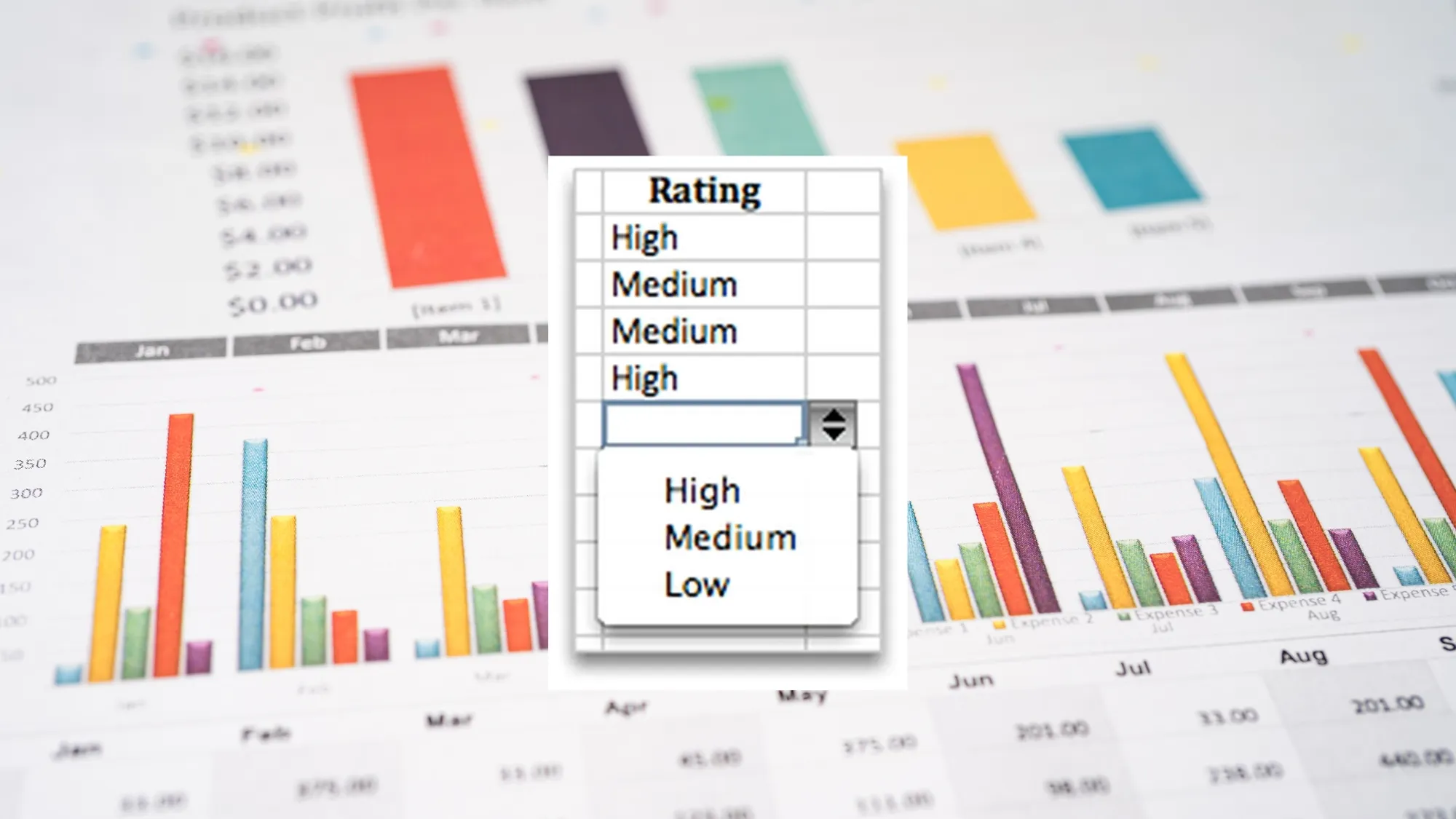
• Prepare Your List: To begin, create a list of valid entries on a sheet. Arrange these entries in the desired order. This list will serve as the source for your drop-down data. If the list is manageable in size, you can input entries directly into the data validation tool.Example: Create a list with entries like High, Medium, and Low.
• Select Cells for Data Entry Restriction: Highlight the cells where you want to apply data entry restrictions.
• Access Data Validation: Go to the Data tab, find Tools, and select Data Validation or Validate.Note: If the validation command is unavailable, your sheet may be protected, or the workbook is shared. You can’t change data validation settings under these conditions.

• Configure Data Validation:
  • Choose the Settings tab.In the Allow pop-up menu, select List.In the Source box, select your list of valid entries from the sheet.
  The dialog box minimizes for better visibility on the sheet.Press RETURN or select the Expand Data validation expand button to restore the dialog box, and then click OK.
  • Tips:
    • You can directly type values separated by a comma into the Source box.To modify the list of valid entries, update the values in the source list or edit the range in the Source box.
    • Bonus Tip: Customize Error Messages Specify your own error message to address invalid data inputs. On the Data tab, select Data Validation or Validate, and then go to the Error Alert tab.

Wrapping It Up

So there you have it, folks! Creating drop-down lists in Excel doesn’t have to be a headache. Whether you’re using Windows or macOS, these steps will help you streamline your data entry processes and keep your data tidy and consistent.

• Also read Honor Magic 6 Pro Hits Malaysia on 20 March, Secure RM2,259 in Early Bird Perks!

And hey, don’t forget to stay tuned to GajetHQ for more tech tips and tricks, especially tailored for our Malaysian audience. Catch ya later!